Perfectly Random
machine learning, probability, and programmingA Guide to Keras Functional API
What is Keras?
Keras means many different things. At the time of writing this article, Keras can refer to one of three things:
- Keras, the API specification
keras, the reference implementation, independent of TensorFlowtf.keras, a particular implementation of the Keras API specification included within TensorFlow
The difference between Keras, the API specification and the Keras implementation (either reference implementation or the TensorFlow implementation) is much like the difference between MPI, the specification and OpenMPI, the particular implementation of MPI.
Keras API specification describes how code can be organized to define and train machine learning models by humans. Keras API specification does not define how the tensor computations are performed at a lower level; that is the job for a deep learning backend such as TensorFlow, Theano, or CNTK.
However, most people understand Keras to be the python package
(keras) that can connect to any of the various deep learning backends.
keras, the python package is a reference implementation
of the Keras API specification. This reference implementation is independent of the
TensorFlow project even though TensorFlow is one of the backends
used by keras. In that sense, keras, the reference implementation may be considered a
wrapper over TensorFlow.
TensorFlow 2.0 adopted Keras API specification as their default, high-level API for building
and training deep learning models. TensorFlow comes with another, self-contained implementation
of the Keras API specification. This implementation is called tf.keras. tf.keras exists
within the tensorflow package and does not require the user to install keras, the reference
implementation. Since tf.keras and keras are both implementations of the same Keras API
specification, there are lots of similarities between tf.keras and keras. But, tf.keras
contains Tensorflow-specific enhancements and may not be exactly the same as keras.
What does this article cover?
In this article, we use the reference implementation,
keras 2.2.4
with TensorFlow backend, to describe the Keras API
specification, specifically, the Functional API.
Most of this article should also apply to tf.keras.
This article aims to provide a deeper understanding of Keras’s inner workings.
The article is intended for audiences who have previously used or attempted to
use a Keras implementation. This article is not an introductory, step-by-step tutorial on how to
use a specific Keras implementation.
Sequential and Functional API
Keras API specification provides two APIs for the end user – Sequential API and the Functional API.
| Sequential API | Functional API | |
|---|---|---|
| Beginner-friendly | Yes | |
| Modeling capability | Directed path graph | Directed acyclic graph |
| Allows multi-input, multi-output models | Yes |
Functional API is much more powerful. Once understood, Functional API is much more intuitive to use. We will discuss only the Functional API in this article.
Keras Objects
Keras API has three fundamental objects, namely:
- Keras Tensor, an augmented version of TensorFlow tensor (when using TensorFlow backend)
- Layer, an object that performs transformation on Keras Tensors
- Model, a specification a neural network, loss functions, optimizers, and other attributes
There are other Keras objects such as Network, Initializer, Optimizer, Callback but the fundamental objects listed above are the only ones important enough to deeply understand Keras. We describe Keras Tensor and Layer in this section and describe Model in the next section.
Keras Tensor
Keras Tensor is commonly generated by the
Input
function, like this:
from keras.layers import Input
x = Input(batch_shape=(10000, 100))
According to the documentation in the code:
A Keras tensor is a tensor object from the underlying backend (Theano, TensorFlow or CNTK), which we augment with certain attributes that allow us to build a Keras model just by knowing the inputs and outputs of the model.
Keras tensor x has the same type as a TensorFlow tensor (since we used TensorFlow
backend), as shown below. However, what makes x a Keras tensor is the existence of
Keras-specific attributes such as _keras_history1.
In [15]: x
Out[15]: <tf.Tensor 'input_1:0' shape=(10000, 100) dtype=float32>

In [16]: type(x)
Out[16]: tensorflow.python.framework.ops.Tensor

In [17]: vars(x)
Out[17]:
{'_op': <tf.Operation 'input_1' type=Placeholder>,
 '_value_index': 0,
 '_dtype': tf.float32,
 '_tf_output': <tensorflow.python.pywrap_tensorflow_internal.TF_Output; proxy of <Swig Object of type 'TF_Output *' at 0x13ff498d0> >,
 '_shape_val': TensorShape([Dimension(10000), Dimension(100)]),
 '_consumers': [],
 '_id': 3,
 '_keras_shape': (10000, 100),
 '_uses_learning_phase': False,
 '_keras_history': (<keras.engine.input_layer.InputLayer at 0x13ff55b38>,
  0,
  0)}
Layer
A Layer defines a transformation. Layer accepts Keras tensor(s) as input, transforms the
input(s), and outputs Keras tensor(s). Layers can do wide variety of transformations.
Dense,
Activation,
Reshape,
Conv2D, and
LSTM are
all Layers derived from the abstract
Layer
class.

A Layer defines a transformation
Typically, we generate a Layer object by calling the default constructor of the corresponding class.
from keras.layers import Dense
dense_layer = Dense(units=10, activation='relu')

In [1]: type(dense_layer)
Out[1]: keras.layers.core.Dense
In the above snippet, dense_layer is an object of the class Dense. Layer objects are
callable because they have a __call__ method2. The __call__ method accepts a
tensor3 or a list/tuple of tensors and returns tensor or a list/tuple of tensors.
Typically, the __call__ method only accepts tensors of shapes that are compatible with its object.
A Layer may or may not have weights associated with it, depending on what it does.
Dense layer does have weights associated with it. However, when using the Functional API,
the weights are not instantiated until we call the dense_layer.__call__() method.
In [2]: # Before calling the __call__ method
    ...: dense_layer.weights
Out[2]: []

In [3]: # After calling the __call__ method
    ...: dense_layer(Input(shape=(100,)))
    ...: dense_layer.weights
Out[3]:
[<tf.Variable 'dense_3/kernel:0' shape=(100, 10) dtype=float32_ref>,
 <tf.Variable 'dense_3/bias:0' shape=(10,) dtype=float32_ref>]
Activation layer, expectedly, does not have any weights associated with it, even after calling
its __call__ method.
In [4]: activation_layer = Activation('relu')

In [5]: activation_layer.weights
Out[5]: []

In [6]: activation_layer(Input(shape=(100,)))
Out[6]: <tf.Tensor 'activation_2/Relu:0' shape=(?, 100) dtype=float32>

In [7]: activation_layer.weights
Out[7]: []
Note about Input and InputLayer
Even though we Input lies within keras.layers, Input is not actually a Layer object.
Input is a function. Calling Input returns a tensor, as we have seen above.
Input
function calls the InputLayer
class, which is indeed a subclass of Layer. InputLayer instantiates a tensor which is
returned to us as the output of the Input function.
Keras Graph
When using a backend (such as TensorFlow), we build a
graph that describes
computation we intend to perform. This graph may be generated implicitly when eager execution
is used or explicitly (such as with sess.run() in TensorFlow).
Even though Keras hides a lot of low-level backend complexity, Keras computation is still based on a graph. Understanding this Keras graph is important to fully understand the Functional API. In fact, by using the Functional API you are specifying a Keras graph. Typically, Keras graph is represented much more compactly than a backend graph. The pictures below show the Keras graph and the corresponding TensorFlow graph for the same network.

Keras graph
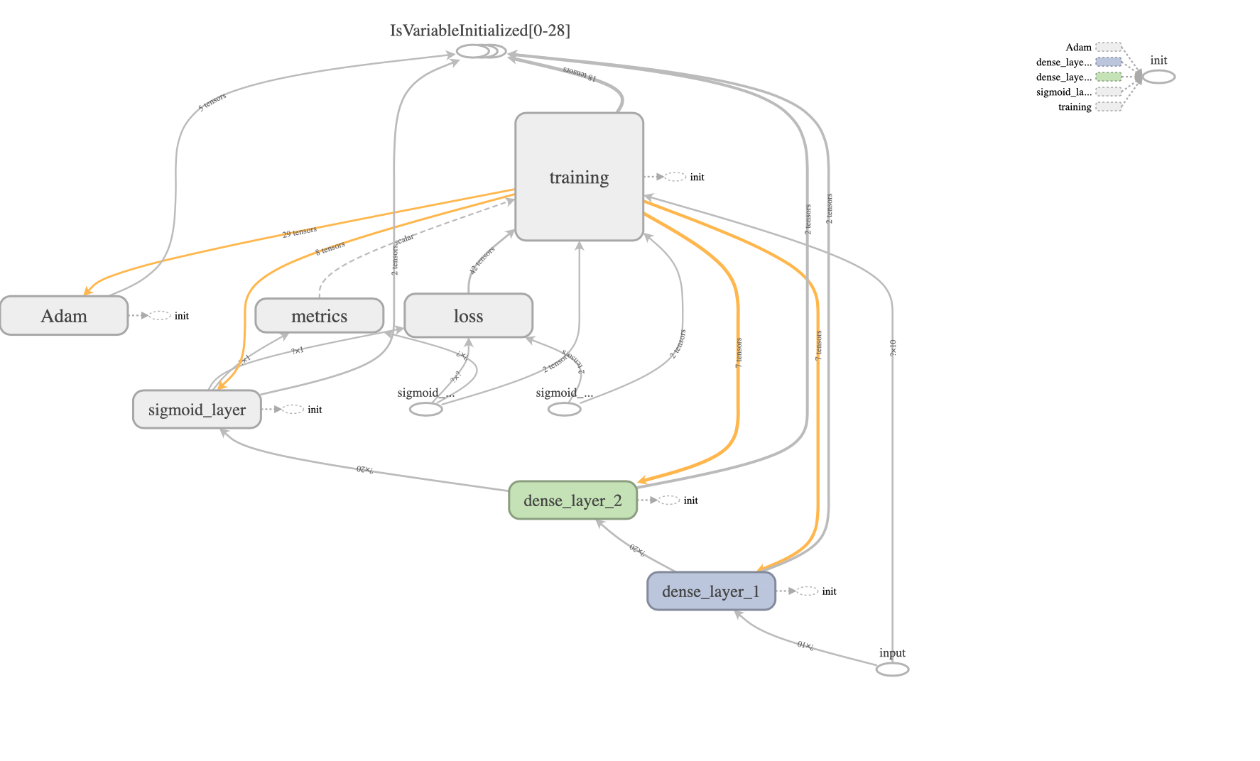
TensorFlow graph
Keras graph construction using Functional API
A graph consists of edges and nodes and Keras graph is no different. Keras graph is a directed
graph4 in which layers act as nodes and tensors act as edges. Specifying the edges is
straightforward – we simply need to create the Layer objects.
from keras.layers import Input, Dense
dense_layer_1 = Dense(units=20, activation='relu', name='dense_layer_1')
dense_layer_2 = Dense(units=20, activation='relu', name='dense_layer_2')
sigmoid_layer = Dense(units=1, activation='sigmoid', name='sigmoid_layer')

# While Input() returns a Keras tensor, Input() implicitly creates an `InputLayer` object
# which acts as a node in the Keras graph.
input_tensor = Input(shape=(10,), name='input')
The above code simply specifies the nodes of the graph. Since we didn’t specify edges just yet, all the nodes are unconnected. We can visualize the current state of the graph as follows.

Keras graph is unconnected until a tensor is flown through it
We can check this using code, as follows. The list of inbound and outbound nodes for
dense_layer_1 are empty. The same is true for dense_layer_2 and sigmoid_layer.
In [3]: dense_layer_1._inbound_nodes
Out[3]: []

In [4]: dense_layer_1._outbound_nodes
Out[4]: []

In [5]: hasattr(dense_layer_1, 'input_shape')
Out[5]: False

In [6]: hasattr(dense_layer_1, 'output_shape')
Out[6]: False
We can also see the dense_layer_1 does not yet have input or input_shape attributes.
Trying to access input_shape attribute gives us the following error.
In [7]: dense_layer_1.input_shape
AttributeError: The layer has never been called and thus has no defined input shape.
Since dense_layer_1 has not been connected to an input yet, it can accept a tensor of any
shape of the form (batch_size, n_units_1, ... ). The output_shape is also undefined at
this stage but will be defined automatically once we provide an input to this layer.
This is a benefit of using Keras – we don’t have to fully specify the input or output shape
of a layer when we instantiate it. The shapes are inferred as we make connections.
The next step is to connect the nodes of the graph with directed edges. This is where the
input_tensor comes into play. The way to connect the nodes is to make a tensor flow through the
nodes5. In the code snippet above, we already created a Keras tensor called input_tensor.
We can now pass6 this tensor through the nodes (layers) using one line of code.
output_tensor = sigmoid_layer(dense_layer_2(dense_layer_1(input_tensor)))
This one line of code connects all the previously unconnected nodes in the order specified.
This results in the following (weakly) connected directed graph.
The InputLayer node is present because of technical reasons and
is typically not important for the end user.

Keras graph is connected once a tensor flows through it
We have now fully specified the Keras graph. We can check that the nodes are connected using code,
just like before. Note that dense_layer_1 now has both input_shape and output_shape
attributes. These shapes were automatically inferred by Keras.
In [3]: dense_layer_1._inbound_nodes
Out[3]: [<keras.engine.base_layer.Node at 0x1129a8d30>]

In [4]: dense_layer_1._outbound_nodes
Out[4]: [<keras.engine.base_layer.Node at 0x136674a20>]

In [5]: hasattr(dense_layer_1, 'input_shape')
Out[5]: True

In [6]: hasattr(dense_layer_1, 'output_shape')
Out[6]: True

In [7]: dense_layer_1.input_shape
Out[7]: (None, 10)

In [8]: dense_layer_1.output_shape
Out[8]: (None, 20)
Model
A neural network is essentially a function which takes input(s) and returns output(s).
In order to fit the neural network represented by the above Keras graph, we need to specify
the input and output to the neural network. These input(s) and output(s) are specified
as list of Keras tensors when initializing a
Model object.
We don’t need to provide any other information about the Keras graph because the input_tensor
and output_tensor edges are already connected to the nodes (layers) of the graph.
from keras.models import Model
model = Model(inputs=[input_tensor], outputs=[output_tensor])
Once we have a Model object, we can specify the optimizer, loss functions, and metrics to track
in the compile step. Model.compile is a method of the class and we don’t need to store its return
value (which is None anyways).
model.compile(optimizer='adam', loss='binary_crossentropy', metrics=['accuracy'])
We haven’t specified the actual (input, output) training data yet. The actual data is
needed only when we fit the model to the training data. Typically, we store the input and
output training data as numpy arrays. These numpy arrays must conform to the shapes of the
input_tensor and output_tensor respectively.
import numpy as np

input_numpy = np.random.rand(1000, 10)
output_numpy = np.random.choice(2, 1000)
The following code snippet shows that the shapes on the actual data (numpy arrays) and the tensors match. The first dimension is always the batch dimension; we will take about this and tensor shapes in detail in the next section.
In [21]: input_numpy.shape
Out[21]: (1000, 10)

In [22]: input_tensor.shape
Out[22]: TensorShape([Dimension(None), Dimension(10)])

In [23]: output_numpy.shape
Out[23]: (1000,)

In [24]: output_tensor.shape
Out[24]: TensorShape([Dimension(None), Dimension(1)])
The only thing remaining is to actually pass the numpy arrays into the model.fit function.
from keras.callbacks import TensorBoard
model.fit(x=[input_numpy], y=[output_numpy],
          epochs=5, batch_size=64, callbacks=[TensorBoard()])
model.fit function accepts an argument x as the input training data. This argument x
requires that we provide a list of numpy arrays in the same order as the list of tensors
specified in the Model’s constructor (i.e., during model instantiation). The same applies to
the y argument.
Tensor shapes
Beginner users find it difficult to correctly specify shapes of tensors and layers. One reason for this is that, in typical usage, Keras doesn’t ask you to provide the shapes of all tensors and layers explicitly upfront; instead, it does shape inference for you. Another reason is that the documentation is vague regarding tensor shapes. Finally, the tensor shapes are different for fully-connected layers, convolutional layers, and recurrent layers.
Batch dimension
This is the most important dimension. Ignoring the batch dimension is also the most common source of error for beginners.
The first dimension is always the batch size, even when the batch size is one.
Batch size is the first dimension even when the "image_data_format": "channels_first".
You cannot ignore the batch dimension even when you have a single (input, output) pair.
For example, if we have some data where the input has 10 features and output is a binary label,
we must specify both the input tensor and input numpy array as 2-dimensional, irrespective of
how many (input, output) pairs we have.
To illustrate this, let’s define a very simple neural network as follows.
def check_batch_size(input_numpy, output_numpy):
    input_tensor = Input((n_features,))
    output_tensor = Dense(units=1)(Dense(units=20)(input_tensor))
    model = Model(inputs=[input_tensor], outputs=[output_tensor])
    model.compile(optimizer='adam', loss='binary_crossentropy',
                  metrics=['accuracy'])
    print(model.summary())
    model.fit(x=[input_numpy], y=[output_numpy], epochs=5)
    return model
Let’s call the check_batch_size function with both the correct and incorrect input shape.
import numpy as np

n_features = 10
batch_size = 1

# Correct
input_numpy = np.random.rand(batch_size, n_features)  # 2-d array
output_numpy = np.random.choice(2, batch_size)        # 1-d array
check_batch_size(input_numpy, output_numpy)  # runs

# Incorrect
input_numpy = np.random.rand(n_features)  # 1-d array
check_batch_size(input_numpy, output_numpy)  # fails because of missing batch dimension
Keras is more forgiving when it comes to the shape of the output_numpy array. But it’s still
a good practice to have batch size be the first dimension in output numpy arrays.
Batch size is not important for neural network specification. This is expected because typically we would like to run the trained model for one test example at a time; fixing the batch size to one particular number would make this difficult. We also often want to try out different (mini) batch sizes during model fitting. When generating an input tensor, Keras lets us choose if we want to specify the batch size up front or wait until the model training stage.
In [6]: Input(shape=(10, ))  # unknown number of examples, each example having 10 features
Out[6]: <tf.Tensor 'input_1:0' shape=(?, 10) dtype=float32>

In [7]: Input(batch_shape=(100, 10))  # 100 examples, each example having 10 features
Out[7]: <tf.Tensor 'input_2:0' shape=(100, 10) dtype=float32>
It is recommended to not specify the batch size up front unless there is a special need.
When we don’t specify the batch size up front, the batch size appears as a ? or None.
In [3]: Input(shape=(10, ))
Out[3]: <tf.Tensor 'input:0' shape=(?, 10) dtype=float32>

In [4]: Input(shape=(10, )).shape
Out[4]: TensorShape([Dimension(None), Dimension(10)])
Convolutional layers
A tensor that interacts with a (2D) convolutional layer has one of two specific shapes.
image_data_format |
Tensor shape |
|---|---|
channels_last |
(batch_size, image_height, image_width, n_channels) |
channels_first |
(batch_size, n_channels, image_height, image_width) |
The image_data_format is typically found in ~/.keras/keras.json.
As an example, for RGB images of 64x64 pixels, we can expect to see something like this:
from keras.layers import Input, Conv2D
input_tensor = Input((64, 64, 3))  # 64x64 pixels, 3 channels
conv_layer = Conv2D(filters=17, kernel_size=(3, 3))
output_tensor = conv_layer(input_tensor)

In [1]: conv_layer.input_shape
Out[1]: (None, 64, 64, 3)

In [2]: conv_layer.output_shape
Out[2]: (None, 62, 62, 17)
Recurrent layers
Typically, recurrent layers such as LSTM accept input of the shape
(batch_size, input_sequence_length, vocab_size). The following examples explain the
two common use cases.
Example 1: One-hot encoded sequence as input
This is the typical case in natural language processing tasks. Given a sentence consisting of five words, we encode the words (text separated by white space) using one-hot encoding. Let’s assume that we only have the four necessary words in the vocabulary.
| 0 | 1 | 2 | 3 | 4 | |
|---|---|---|---|---|---|
| Sentence | the | cat | and | the | dog |
| Encoding | [0, 1, 0, 0] |
[1, 0, 0, 0] |
[0, 0, 1, 0] |
[0, 1, 0, 0] |
[0, 0, 0, 1] |
In this case, the input sequence length is 5 and the size of each element of the input sequence
is a one-hot vector of length 4. Thus, one input example is of size
(input_sequence_length, vocab_size) = (5, 4) and there can be many input examples in a batch.
The following code represents how to build an LSTM model to accept this input.
from keras.layers import Input, LSTM, Dense

input_sequence_length = 4
vocab_size = 5
input_tensor = Input(shape=(input_sequence_length, vocab_size))
lstm_layer = LSTM(units=10, return_sequences=False, return_state=False)
dense_layer = Dense(vocab_size, activation='softmax')
output_tensor = dense_layer(lstm_layer(input_tensor))
Note how we have set return_sequences and return_state to be False.
The output of the lstm_layer is a tensor of shape (batch_size, n_lstm_units) = (None, 10).
In [30]: lstm_layer.output_shape
Out[30]: (None, 10)
Changing any of the arguments return_sequences and return_state to True would change
the output shape completely7.
Example 2: Scalar, real-valued sequence as input
This example is in contrast to the previous example. This time, let us assume that we are trying to model a sequence of scalar, real-valued quantities. One example could be the stock price of one particular stock. We want a model that takes as input a sequence of 5 stock prices and outputs the next (6th) stock price. There is no need to encode the real-valued stock price8. The input data looks like this:
| 0 | 1 | 2 | 3 | 4 | |
|---|---|---|---|---|---|
| Price | 30.56 | 29.54 | 32.12 | 36.78 | 40.01 |
Even though the stock price is a scalar quantity, for LSTM, we will have to consider the stock price to be a vector of one dimension. The following code snippet shows the correct and incorrect way of specifying tensor shapes.
from keras.layers import Input, LSTM, Dense

# Correct
input_sequence_length = 5
input_dimension = 1
input_tensor = Input(shape=(input_sequence_length, input_dimension))
lstm_layer = LSTM(units=10, return_sequences=False, return_state=False)
dense_layer = Dense(input_dimension, activation='softmax')
output_tensor = dense_layer(lstm_layer(input_tensor))  # runs

# Incorrect
input_sequence_length = 5
input_tensor = Input(shape=(input_sequence_length,))
lstm_layer = LSTM(units=10, return_sequences=False, return_state=False)
dense_layer = Dense(1, activation='softmax')
output_tensor = dense_layer(lstm_layer(input_tensor))  # fails
Batch normalization layer
BatchNormalization layer is another common reason for shape-related errors.
Batch normalization was proposed by Ioffe & Szegedy, 2015 primarily for fully-connected (Dense) layers and convolutional layers. The authors mention that at the time they did not fully explore the application of batch normalization to recurrent neural networks (see Page 8, last paragraph, Ioffe & Szegedy, 2015). In the subsequent years, various other forms of normalization methods were proposed including Layer Normalization by Lei Ba et al., 2016 and Recurrent Batch Normalizaton by Cooijmans et al., 2016. Local Response Normalization, which is a normalization over channels in convolutional layers, was proposed by Krizhevsky et al., 2012.
The batch normalization performed by the
BatchNormalization
function in keras is the one proposed by Ioffe & Szegedy, 2015 which is
applicable for fully-connected and convolutional layers only9.
The key to the BatchNormalization layer in keras is the axis argument, which has a rather
confusing documentation, as discussed in this
StackOverflow post.
As described in this post, the confusion arises because numpy functions (such as np.mean) also
have an axis argument and the meaning of axis in np.mean is opposite to that in
BatchNormalization. In np.mean, the axis argument indicates the axis that is to be
collapsed. In BatchNormalization, axis argument indicates the axis that is to be preserved.
Fully-connected layers
Let’s consider the following simple examples. The input tensor to BatchNormalization
consists of three examples in a batch; each example in the batch has 2 features.
from keras.layers import Input, BatchNormalization

batch_size = 3
n_features = 2
input_tensor = Input(batch_shape=(batch_size, n_features))

# Example 1: average over batches (typically correct)
output_tensor_1 = BatchNormalization(axis=1)(input_tensor)  #runs

# Example 2: average over features (typically incorrect)
output_tensor_2 = BatchNormalization(axis=0)(input_tensor)  #runs
Example 1 in the snippet above computes mean and variance for each of the two features independently. While computing the mean and variance for one particular feature, Example 1 averages over the three batches – it computes the mean of three scalar numbers.
Example 2 in the snippet above computes mean and variance for each of the three examples in the batch independently. While computing mean and variance for one particular example, Example 2 average over the two features – it computes the mean of two scalar values.
Even though the two examples perform meaningfully different computations, the shape of the output tensor remains the same.
In [1]: output_tensor_1
Out[1]: <tf.Tensor 'batch_normalization_2_1/cond/Merge:0' shape=(3, 2) dtype=float32>

In [2]: output_tensor_2
Out[2]: <tf.Tensor 'batch_normalization_2_2/cond/Merge:0' shape=(3, 2) dtype=float32>
Thus, there is no way for us (or for Keras) to check if we have used the correct value for
axis! Typically, when we perform batch normalization, we would like to average over batches
and not features. Therefore, Example 1 is the more typical usage (by far) and represents the correct
way to perform the commonly understood implementation of batch normalization.
The problem becomes worse when we have more than one feature dimension, as shown below.
from keras.layers import Input, BatchNormalization

batch_size = 3
feature_shape = (2, 4, 5)
input_tensor = Input(batch_shape=(batch_size,) + feature_shape)

# Example 1
output_tensor_1 = BatchNormalization(axis=1)(input_tensor)

# Example 2
output_tensor_2 = BatchNormalization(axis=2)(input_tensor)

# Example 3
output_tensor_3 = BatchNormalization(axis=3)(input_tensor)
As before, all the three output tensors in the snippet above have the same shape. Thus, we cannot use the shape of the output tensor to determine which one of the three batch normalizations is the correct one. The input tensor has the same shape as the output tensors.
In [3]: input_tensor
Out[3]: <tf.Tensor 'input_1:0' shape=(3, 2, 4, 5) dtype=float32>
Example 1 would preserve the second dimension (=2) of the input tensor and average over all
the rest. Example 2 would preserve the third dimension (=4). Example 3 would preserve the
fourth dimension (=5).
There is no easy way10 for us to preserve more than one dimension at a time when using
BatchNormalization.
Convolutional Layers
The underlying code for BatchNormalization is the same whether it’s used for fully-connected
layers or for convolutional layers. But, for convolutional layers, we need to consider
the image_data_format when deciding the value of axis argument for BatchNormalization.
The following table shows the usual values of the axis argument
for both options of image_data_format.
image_data_format |
Tensor shape | axis |
|---|---|---|
channels_last |
(batch_size, image_height, image_width, n_channels) |
axis=3 |
channels_first |
(batch_size, n_channels, image_height, image_width) |
axis=1 |
For both of the cases above, BatchNormalization would preserve the channel dimension and average
over the rest. This means that we would average over all the examples in the batch as well
as the all of the pixels, together. While this may look like a mistake, this is actually correct.
This behavior is actually what Ioffe & Szegedy, 2015 specified in
their implementation for convolutional layers (see Section 3.2, last paragraph
in Ioffe & Szegedy, 2015).
The authors desired that the normalization obey the convolutional property
such that different elements of the same feature map (i.e., channel) at different locations
are normalized in the same way.
Final thoughts
Keras is an excellent high-level API to build neural network models. Keras Functional API is powerful enough to let us build complicated models without having to descend into the low-level, backend API. While Keras documentation is vague at times, Keras provides sensible defaults and performs shape inference to discover mistakes at model specification time. I hope that this post provides some help with the vaguely documented sections of the Keras codebase and saves you some time and effort. If you notice any mistakes or areas that I have overlooked, please leave a comment and let me know.
Footnotes
-
According to the
is_keras_tensorfunction, an object is a Keras tensor if it is a backend tensor and has the_keras_historyattribute. ↩ -
This is not a Keras-specific functionality. In python, an object can be made callable by adding a
__call__method to it. For example:class Example(object): def __init__(self, data): self.data = data def __call__(self, *args, **kwargs): return self.data x = Example(1) In [1]: x(2) Out[1]: 1 In [2]: x() Out[2]: 1 -
Either a Keras tensor or a backend tensor. ↩
-
Edge directions in a Keras graph indicate the forward pass of the neural network. During the backward pass or backpropagation, which computes the gradients, we reverse all edges of the graph to get the transpose graph. ↩
-
And, so, TensorFlow earns its name. ↩
-
Much like threading pearls (
Layerobjects) with a string (Keras tensor). ↩ -
Tensor handling by
LSTM,SimpleRNN, andGRUare a subject for a future post. ↩ -
In a real application, we may need to scale the (real) values into a bounded range such as
[-1, 1]. We omit the rescaling discussion because it doesn’t affect the conclusion. ↩ -
I do not recommend using
BatchNormalizationfor recurrent layers, unless you know what you’re doing. Based on the code, theaxisargument toBatchNormalizationis not general purpose. It is specifically designed to match the implementation described in Ioffe & Szegedy, 2015, which is only applicable for fully-connected and convolutional layers. ↩ -
We could always use
keras.layers.Lambdaandkeras.layers.Reshapeto extract and reshape individual dimensions and perform the normalization ourselves. ↩