Perfectly Random
machine learning, probability, and programmingBernoulli Distribution as a tiny Neural Network
Logistic regression is often considered the smallest neural network for binary classification. We can think of Bernoulli distribution as an even smaller neural network – one that doesn’t even depend on the input data. Such a neural network would likely not be useful in practice. However, given it’s simplicity, it serves as an illuminating example to help us understand the statistical assumptions underlying a neural network model. The assumptions we require for modeling Bernoulli distribution as a neural network are also required for larger neural networks. As an example, using Bernoulli distribution as a tiny neural network, we can easily demonstrate how the famous cross-entropy loss comes into being. We can even extend this Bernoulli distribution model framework to recreate the familiar logistic regression model by simply replacing a constant parameter by a sigmoid-affine function.
(This document is available as a PDF)
Bernoulli distribution
Bernoulli distribution, owing to its simplicity, is used more often than it is noticed. A random variable \(X \sim \text{Bernoulli}(p)\) has the following probability mass function (pmf):
\[\begin{aligned} P(X = 1) &= p \notag \\ P(X = 0) &= 1 - p \label{eqn:raw-form}\\ P(X \notin \{0, 1\}) &= 0 \notag \end{aligned}\]in which, the only parameter, \(p\), is a probability and therefore must satisfy \(0 \le p \le 1\). We call the above equation the raw form pmf of the Bernoulli distribution.
The raw form pmf is simple to understand but its multi-case structure makes it difficult to use in other derivation. We can combine the two of the three cases into one equation without changing anything about the distribution. This results in the following two forms of pmf – the additive form:
\[P(X = x) = \begin{cases} p x + (1 - p) (1 - x) & x \in \{0, 1\} \\ 0 & \text{otherwise} \end{cases} \label{eqn:additive-form}\]and the multiplicative form:
\[P(X = x) = \begin{cases} p^x (1 - p)^{(1 - x)} & x \in \{0, 1\} \\ 0 & \text{otherwise} \end{cases} \label{eqn:multiplicative-form}\]All three forms — raw, additive, multiplicative1 — are equivalent to each other and represent the same exact distribution. This implies that no matter which of the three forms we use for our analysis, we should get the exact same analytical result. However, one form may be easier to work with than the others when wrangling algebraic equations. The multiplicative form is the most common one used in both statistical analysis and with neural networks.
Binary classification
Let’s consider a familiar application of supervised binary classification in computer vision – image classification. We would like to classify a given image into one of two classes – a cat image versus a dog image:
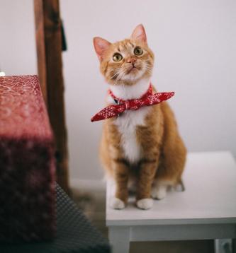
Cat
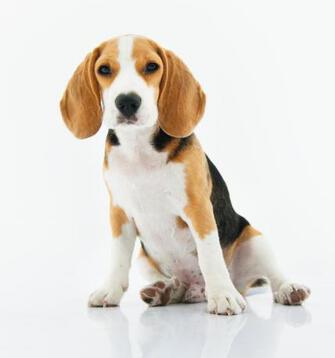
Dog
Image by Pexels
In a supervised setting, we usually have training data available, which is represented as:
\[\{ (x^{(1)}, y^{(1)}), (x^{(2)}, y^{(2)}), \ldots, (x^{(i)}, y^{(i)}), \ldots, (x^{(m)}, y^{(m)}) \} \label{eqn:binary-classification-data}\]in which, \(x^{(i)} \in \mathbb{R}^{n_x}\) is the input data and \(y^{(i)} \in \{0, 1\}\) is the output label. For the cat vs dog example, \(x^{(i)}\) is a vector of pixel values obtained by flattening the tensor that represents an image and \(y^{(i)}\) represents the label – cat (\(y=1\)) or dog (\(y=0\)).
Modeling the binary classification problem as Bernoulli distribution
Modeling binary classification
We aim to fit a function to describe the input-output relationship in the training data. We could attempt to find a suitable deterministic function \(y=f(x, \theta)\) and minimize (w.r.t the model parameters \(\theta\)) some appropriate measurement of discrepancy (\(\Phi(\theta)\)) between the function’s predicted labels and true labels2. Alternatively, we could model the output label as a random variable3
\[Y\sim\text{SomeDistribution}(x, \theta) \label{eqn:some-distribution}\]in which, \(\theta \in \mathbb{R}^{n_t}\) is the set of model parameters. The training data (shown above) is interpreted as a list of \(m\) statistical samples of \(Y\) generated along with the corresponding values of \(x\).4 When we choose to model the output label as random variable, we have a well-established approach to minimize the discrepancy between the predicted and true labels – maximum likelihood estimation.
Modeling with Bernoulli distribution
Since the true output labels only take values in \(\{0, 1\}\), it would be ideal if our choice of random variable also assumes values in \(\{0, 1\}\). Bernoulli distribution is one such choice:
\[Y\sim\text{Bernoulli}(p) \label{eqn:bernoulli-model}\]in which, \(\theta = \begin{bmatrix}p\end{bmatrix}\). Note how the model above doesn’t depend on the input \(x\) at all.
Now that we have a statistical model to describe the output, we can write down the likelihood as follows:
\[\begin{aligned} &\mathcal{L}(\theta) \notag\\ &= P\left( (Y^{(1)} = y^{(1)}) \cap (Y^{(2)} = y^{(2)}) \cap \ldots (Y^{(i)} = y^{(i)}) \cap \ldots (Y^{(m)} = y^{(m)}) ; \theta \right) \label{eqn:likelihood}\\ &= P\left( (Y^{(1)} = y^{(1)}) \cap (Y^{(2)} = y^{(2)}) \cap \ldots (Y^{(i)} = y^{(i)}) \cap \ldots (Y^{(m)} = y^{(m)}) \mid \Theta = \theta \label{eqn:likelihood-bayesian} \right)\end{aligned}\]The second equation is the Bayesian form of likelihood, in which we choose to model the parameters as a random variable \(\Theta\). The first equation is also the likelihood but it doesn’t consider the model parameters as random variables. We will only use the first form of likelihood in this document because we have no need to model the parameter(s) as random variable(s) at this time.
Assuming independence, we can re-write the likelihood as:
\[\mathcal{L}(\theta) = \prod_{i=1}^{i=m} P\left( Y^{(i)} = y^{(i)} ; \theta \right)\]Substituting the multiplicative form and applying the knowledge that the output labels \(y^{(i)} \in \{0, 1\}\), we obtain:
\[\mathcal{L}(\theta) = \prod_{i=1}^{i=m} p^{y^{(i)}} (1 - p)^{(1 - y^{(i)})} \label{eqn:multiplicative-likelihood}\]Taking logarithm, the log-likelihood is:
\[\log \mathcal{L}(\theta) = \sum_{i=1}^{i=m} \left[ y^{(i)}\log p + (1 - y^{(i)})\log (1 - p) \right] \label{eqn:bernoulli-log-likelihood}\]The expression above is the famous cross-entropy loss5. Maximizing the log-likelihood:
\[\begin{aligned} 0 &= \frac{\partial \log \mathcal{L}(\theta)}{\partial p} \notag \\ 0 &= \sum_{i=1}^{i=m} \left[ \frac{y^{(i)}}{p} - \frac{(1 - y^{(i)})}{(1 - p)} \right] \notag \\ \implies \hat{p} &= \frac{\sum_{i=1}^{i=m} y^{(i)}}{m} \end{aligned}\]in which \(\hat{p}\) is the maximum likelihood estimate for \(p\). In order to confirm that this value of \(\hat{p}\) actually maximizes the log-likelihood, we can show that the second order derivative is negative as follows:
\[\begin{aligned} \frac{\partial^2 \log \mathcal{L}(\theta)}{\partial p^2} = - \sum_{i=1}^{i=m} \left[ \frac{y^{(i)}}{p^2} + \frac{(1 - y^{(i)})}{(1 - p)^2} \right] < 0 \end{aligned}\]See Appendix A in the PDF version for the same result obtained using the additive form.
Extension to logistic regression
In the previous subsection, we didn’t even consider the input \(x\) in our model. If we want to include the input \(x\), we could replace the previously constant \(p\) with a function of \(x\). A simple way to include \(x\) is to model \(p\) as an affine6 function of \(x\) instead of a constant
\[p = w^{T} x + b \label{eqn:affine}\]in which, \(w \in \mathbb{R}^{n_x}\) and \(b \in \mathbb{R}\) are model parameters. However, there is a problem with the above affine function – there is no guarantee that the expression \(w^{T} x + b\) would be within \(0\) and \(1\), as required for \(p\).7 We can solve this problem easily by passing \(w^{T} x + b\) through a sigmoid function to obtain the following sigmoid-affine function:
\[\begin{aligned} p = \sigma(w^{T} x + b) \\ \sigma(z) = \frac{1}{1 + e^{-z}} \label{eqn:sigmoid} \end{aligned}\]The resulting model for \(Y\) becomes:
\[Y \sim \text{Bernoulli}(\sigma(w^{T} x + b))\]which is exactly the logistic regression model. The difference is that instead of directly assuming the logistic form, we have chosen to interpret logistic regression model as an extension of the Bernoulli distribution.
We can now perform log-likelihood maximization as usual. The likelihood is given by the following expression:
\[\begin{aligned} &\mathcal{L}({\theta})\notag\\ &= P\left( (Y^{(1)} = y^{(1)}) \cap (Y^{(2)} = y^{(2)}) \cap \ldots (Y^{(i)} = y^{(i)}) \cap \ldots (Y^{(m)} = y^{(m)}) ; \theta \right) \notag \\ &=\prod_{i=1}^{i=m} P\left( Y^{(i)} = y^{(i)} ; \theta \right) \quad \text{(independence)} \notag \\ &=\prod_{i=1}^{i=m} \left[ \{\sigma(w^{T} x + b)\}^{y^{(i)}} \{1 - \sigma(w^{T} x + b)\}^{(1 - y^{(i)})} \right] \quad (y^{(i)} \in \{0, 1\}, \text{for all } i) \end{aligned}\]in which, \(\theta = \begin{bmatrix}w & b\end{bmatrix}\). The log-likelihood may be written as:
\[\begin{aligned} \log \mathcal{L}(\theta) = \sum_{i=1}^{i=m} \left[ y^{(i)}\log \sigma(w^{T} x + b) + (1 - y^{(i)})\log (1 - \sigma(w^{T} x + b)) \right] \label{eqn:logistic-log-likelihood} \end{aligned}\]Log-likelihood may be maximized via any of the numerical optimization algorithms such as gradient descent.
Summary
Log-likelihood equations for Bernoulli distribution and logistic regression have the same form. In fact, we can obtain the log-likelihood for logistic regression by simply replacing the \(p=\sigma(w^{T}x + b)\) in the log-likelihood for the Bernoulli model. Logistic regression is a one-layer8 neural network:

Logistic Regression
We can think of the Bernoulli model as an even simpler neural network that isn’t connected to the input layer at all:

Bernoulli Model
Equivalently, Bernoulli model is the same as a logistic regression model that has all the weights \(w\) set to zero and \(p=\sigma(b)\). Bernoulli model has a constant number of unknown model parameters while logistic regression has a parameter linear complexity in the input image size. Conversely, we can also think of logistic regression as one particular extension of the Bernoulli model framework.
Footnotes
-
Note that we interpret \(0^0\) as \(1\) and \(\log 0^0 = 0\log0 = 0\). ↩
-
For certain choices of \(f(x, \theta)\) and \(\Phi(\theta)\), the estimated model parameters may equal the estimated model parameters obtained using the statistical modeling approach, analytically. ↩
-
A random variable is also a function (a measurable function) but we choose to highlight the difference between any deterministic function and the restrictive measurable function that is a random variable. ↩
-
For this problem, we choose to consider the list of different images (i. e., \(x\)’s) as deterministically fixed. Therefore, \(x\) is not random and we do not condition on \(x\). ↩
-
This is a demonstration of the equivalence between maximizing the likelihood and minimizing the KL divergence. ↩
-
A linear function \(p = w^{T}x\) would be even simpler than affine function \(p = w^{T} x + b\). ↩
-
We could always treat the problem as a constrained optimization problem in which \(w, b\) can only take values such that \(0 \le w^{T} x + b \le 1\) but we do not pursue this line of analysis. ↩
-
Typically, we don’t count input layer at all. ↩